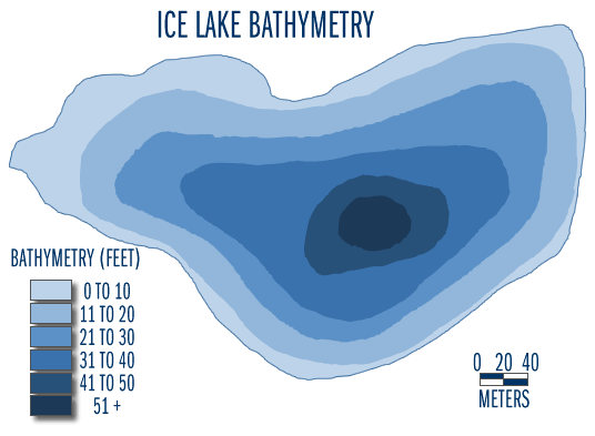
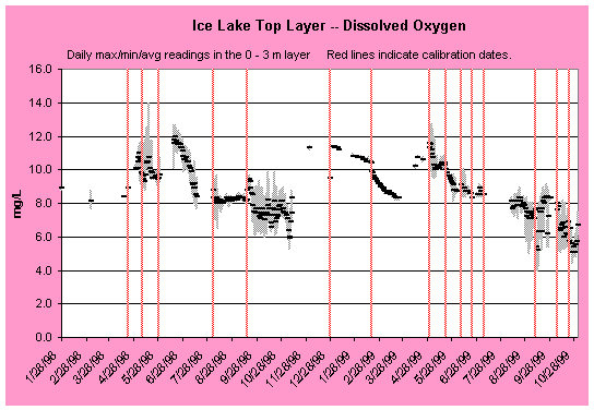
RUSS Data Ice Lake (http://wow.nrri.umn.edu/wow/data/ice/current.html)
Water on the Web's data archive is integrated
in a domain Data
that contains data as well as tools for their visualization. A start
page (http://wow.nrri.umn.edu/wow/data.html)
allows the user to select one of the six lakes, and the information about
that lake they would like to see. The available information about the lakes
are portioned into four domains:
| - | RUSS Data: | raw data, data from the measurement of the RUSS Unit |
| - | Data Visualization: | graphic online tools |
| - | Environmental Data: | information about environment of the respective lake |
| - | Lake Trends: | already organized and aggregated data, partly enriched with graphical displays |
Below we present the data sets and visualization tools related to these four domains.
RUSS Data Ice Lake (http://wow.nrri.umn.edu/wow/data/ice/current.html)
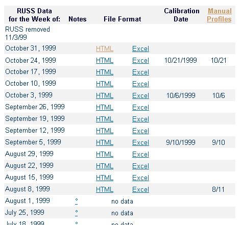
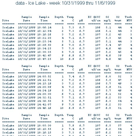
Below we show the data in HTML format.
Weekly RUSS data, HTML Format
(http://wow.nrri.umn.edu/wow/data/ice/russ/ice19991031.html)
The Excel tables contain all variables included in the HTML tables as
well as the additional variables: schedule depth (the depth that
they hoped to sample at) and actual depth (the actual depth sampled). These
two can differ by up to 0.2 m. An advantage of the Excel spreadsheets
is that they contain prepared graphs, which we further describe in our
Chapter on Tools
for Data Analysis.
The "complete archive" tables are only minimally different from the
"weekly Excel tables": only a column with "scheduled time" was added, which
is the time the measurement was scheduled to be taken.
|
|
|
|
|
Depth |
Depth |
|
|
|
|
|
|
|
|
|
|
|
|
|
|
|
|
|
|
|
|
|
|
|
|
|
|
|
|
|
|
|
|
|
|
|
|
|
|
|
|
|
|
|
|
|
|
|
|
|
|
|
|
|
|
|
|
|
|
|
|
|
|
|
|
|
|
|
|
|
|
|
|
|
|
|
|
|
|
|
|
|
|
|
|
|
|
|
|
|
|
|
|
|
|
|
|
|
|
|
|
|
|
|
|
|
|
|
|
|
|
|
|
|
|
|
|
|
|
|
|
|
|
|
|
|
|
|
|
|
|
|
|
|
|
|
|
|
|
|
|
|
|
|
|
|
|
|
|
|
|
|
|
|
|
|
|
|
|
|
|
|
|
|
|
|
|
|
|
|
|
|
|
|
|
|
|
|
|
|
|
|
|
|
|
|
|
|
|
|
|
|
|
|
|
|
|
|
|
|
|
|
|
|
|
|
|
|
|
|
|
|
|
|
|
|
|
|
|
|
|
|
|
|
|
|
|
|
|
|
|
|
|
|
|
|
|
|
|
|
|
|
|
|
|
|
|
|
|
|
|
|
|
|
|
|
|
|
|
|
|
|
|
|
|
|
|
|
|
|
|
|
|
|
|
|
|
|
|
|
|
|
|
|
|
|
|
|
|
|
|
|
|
|
|
|
|
|
|
|
|
|
|
|
|
|
|
|
|
|
|
|
|
|
|
|
|
|
|
|
|
|
|
|
|
|
|
|
|
|
|
|
|
|
|
|
|
|
|
|
|
|
|
|
|
|
|
|
|
|
|
|
|
|
|
|
|
|
The description
page gives short explanations for all 12 variables of the "complete
data":
|
|
Lake | It is an abbreviation of the site name. |
| - | SchedDate | The scheduled date for the reading. |
| - | SchedTime | All the readings for a given profile have the same SchedTime and SchedDate. |
| - | ActDateTime | The actual date and time the reading was made. |
| - | SchedDepth | The depth in meters where the reading is scheduled to occur. |
| - | ActDepth | The depth in meters where the reading actually was made. |
| - | Temp | The temperature in degrees Celsius. |
| - | pH | The pH value. |
| - | Cond | The electrical conductivity in microSiemens/cm. |
| - | DO | Dissolved oxygen in mg/L. |
| - | DOpctSat | Dissolved oxygen % saturation at temperature. |
| - | Turb | The turbidity in NTUs. |
The last six variables link to explanations which include why values on that variable vary and its potential impact on pollution.
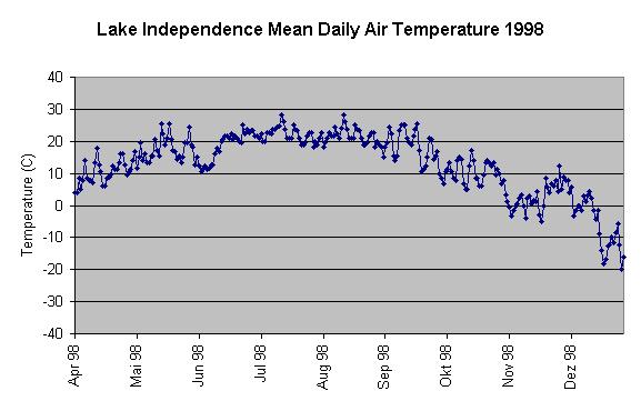
(http://wow.nrri.umn.edu/wow/data/independence/spreadsheet/indy_weather1998.xls)
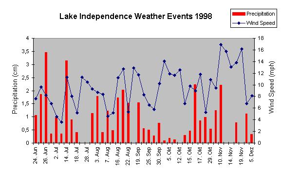
The other prepared graph is a time series of major weather events (precipitation and wind speed). Again, we show as an example below the graph for Lake Independence in 1998. (The graph for Ice Lake includes precipitation only.)
(http://wow.nrri.umn.edu/wow/data/independence/spreadsheet/indy_weather1998.xls)
The above graph has several deficiencies. First, the time axis is not an adequate continuous axis of time. The first three columns belong to three successive days (June 24th to June 26th), while the fifth column represents July 5th, and so on. This problem occurs if one uses Excel without caution in which case the x-axes is interpreted by Excel as a category axis. A second problem is that the values of wind speed are drawn as a line graph. The slopes can be misleading because the time intervals between two points differ in their length. Wind speed was measured only on particular days, namely when either it was windy (above a certain limit) or rain fell. The wind on the days between was definitely lower, and therefore the lines connecting the points are additionally misleading. Anyway, we have reproduced the graph elsewhere and the diagnosis of a trend remains true at least related to the selected points of measurement. One reason of the problem is that EXCEL cannot adequately deal with missing data, another source is how to deal with measurements that are always selected at certain points in time and have to asked how "representative" they are.
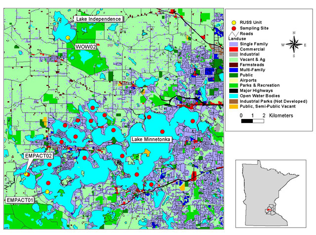
The landuse maps (see example below) are typically color-coded and show how the land surrounding the lake is being used (see key below for usage categories).
Many types of data are needed to characterize the ecology of lakes and streams and a variety of techniques are available for best presenting them. This section includes graphs of various parameters plotted over time or versus depth and tabular summaries of other parameters, such as water chemistry, secchi transparency, chlorophyll, etc.
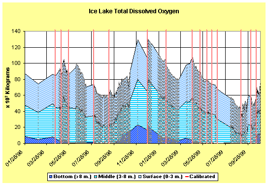
The RUSS data from Lake Independence is summarized to
show the lake's average heat and oxygen content on each day. These are
calculated by averaging the amount of heat and oxygen contained in each
1 meter thick layer of the lake over the course of the day and then adding
them up from 0-3 m, 3-8 m and 8 meters to bottom. Therefore, the sum of
the values for the 3 layers is the total amount in the whole lake on that
day. Limnologists say that these values are morphometrically-, or
volume-weighted.
Charts of heat and oxygen content are provided below.
These are "stacked-area" charts - showing the contribution of each layer
to the total. Below each chart you will find a more detailed description
of the calculations involved for determining the heat content and oxygen
content. (http://wow.nrri.umn.edu/wow/data/independence/heat.html)
(The vertical lines indicate the calibration dates):
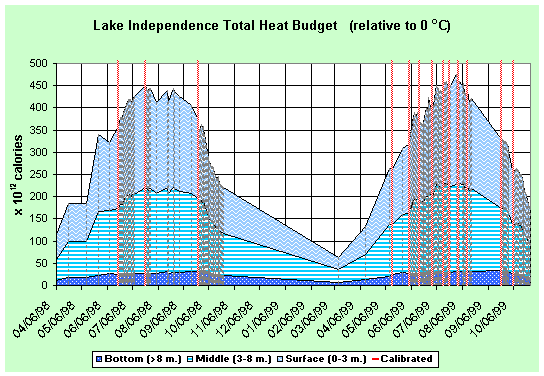
The graphs exemplarily show what is expected from students.
We also present the reconstruction in our report with great detail, because we want to show the complex definition of variables as one feature of the project and its data.
Heat budget is computed using the following formula:
heat content = mass * specific heat * temperature = m * C * delta T . Mass is calculated by mass = volume * density
The calculation of the dissolved oxygen is done in a similar way.
There is an assumption being made here that we think should be pointed
out to students. The materials tell the students that "Water has
a specific heat of 1.0 calories per gram per degree Celsius. This means
that it takes 1 calorie of heat energy to raise the temperature of a gram
of water by 1°C." However, heat content is a relative magnitude related
to a certain zero-level of temperature. The variable temperature
in the above formula, in essence, is a temperature difference. The authors
relate the temperature to 0 ° C as we can also see from the graph.
That is why temperature and temperature difference have equal values here,
although there is an important conceptual difference.
The authors say that density = 1 gram/milliliter = 1 kg/liter. The authors do not point out here that density is dependent on the temperature of the water. We think that it is all right to ignore these differences because they will have only a minimal influence on the result. However, it would have been better to mention this dependence and to argue that it is reasonable to ignore these differences. This is important because these differences become significant in other parts of the project, because the structures of the water layers are influenced by this property. The authors could have mentioned the chapters on Density Stratification in the Lake Ecology primer. There, this anomaly of water (maximum density at 4 ° C) is shown by a graph. This anomaly accounts for why fish can survive in frozen lakes.
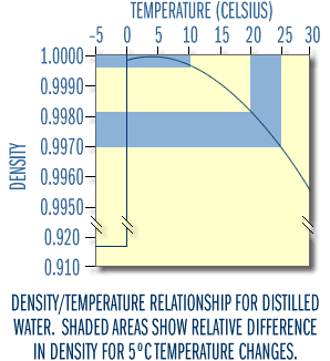
(http://wow.nrri.umn.edu/wow/under/primer/art/densityvstemp.gif)
As an example, the authors' show the calculation of the heat content of the upper layer of Ice Lake for May 29th, 1998, at 6 a.m. They show the following table beside the above formula.
|
|
(x 105 m3) |
(average of layer) |
(calories per layer) |
| 0-1 meters | 1.60 | 20.80 | 3.33 x 10¹² |
| 1-2 meters | 1.48 | 20.75 | 3.07 x 10¹² |
| 2-3 meters | 1.36 | 19.55 | 2.66 x 10¹² |
| Total (0-3 m) | 4.44 |
|
They do not say how they computed average temperature of a layer, but it appears that they get this by taking the mean of the upper and lower border of the layer.
It is more difficult to understand how the volume of the different layers
of the Ice Lake was determined. We find some information about volume under
the point "morphometry" which can be found via the data archive. We can
read the following:
To estimate the area at the top of any layer, use the
following formula:
Regression of: Area (hectares) at top of layer vs depth
of layer top (meters)
where area(ha) is for the top of the layer and z is the depth in meters at the middle of the layerA(z) = (-1.184)*z + 16.58
where V(z) is the volume of the layer.V(z) = (-0.113)*z + 1.633
We found no information about how these formulae were derived. It would be an interesting task to interpret these formulae and to analyze assumptions that were made. For the first formula (area) a simple interpretation is that we have a volume like a square stone with a slanting side which has a slope of (-1,184). The result for z=0 is the surface area of the Ice Lake, and it accords with the information of the lake summary table. We did not find any information about the formula of the volume. Given that the authors did not use this formula, we can surmise that they themselves do not trust it. We have calculated the layer volume according to this formula and show this in the table by means of an added column. We see that the values differ, although the difference is not very large, between the depth of zero and nine meters. With the following formula you get the same results as in the table:
| Table
2
Complete depth profiles of area (at top of layers) and layer volumes for Ice Lake. z1 and z2 refer to the top and bottom depths of a particular layer. |
||||
|
Z (meters) |
@ top (hectares) |
z1 to z2 (m) |
(x106 m3) |
|
| 0 | 16.6 | 0-1 | 1.600 | 1.5765 |
| 1 | 15.4 | 1-2 | 1.481 |
|
| 2 | 14.2 | 2-3 | 1.362 |
|
| 3 | 13.0 | 3-4 | 1.244 |
|
| 4 | 11.8 | 4-5 | 1.126 |
|
| 5 | 10.7 | 5-6 | 1.008 |
|
| 6 | 9.49 | 6-7 | 0.889 |
|
| 7 | 8.30 | 7-8 | 0.771 |
|
| 8 | 7.11 | 8-9 | 0.652 | 0.6725 |
| 9 | 5.93 | 9-10 | 0.534 |
|
| 10 | 4.75 | 10-11 | 0.416 |
|
| 11 | 3.57 | 11-12 | 0.297 |
|
| 12 | 2.38 | 12-13 | 0.179 |
|
| 13 | 1.20 | 13-14 | 0.063 |
|
| 14 | 0.060 | 14-15 | 0.004 |
|
| 15 | 0.029 | 15-16 | 0.001 |
|
| Total Volume = | 11.6 (x105 m3) | |||
If we trust the values of the table we now can reconstruct the calculation now.