Our analysis is based on the current state of the curriculum, which is still under development. Various tools such as the color mapper and the DxT profiler have only recently become available and are not integrated into the units. Therefore this should not be read as a final evaluation of the units, as they are still under revision. Indeed, as we were preparing this report, we contacted the authors about problems we had encountered and they were quick to respond and to revize their materials accordingly.
The information for teachers in the chapter on "procedure" differs for the studying lessons and for the investigating lessons.Goals Introduction Outcomes Keywords Materials/Resources/Software Time Required Curriculum Connections Procedure
- Knowledge Base
- Experimental Design
- Data Collection
- Data Management and Analysis
- Interpretation of Results
- Reporting ResultsResources Extensions
pH:Note that decomposition decreases pH as well DO. This fact will be important in understanding the results of our own analysis, reported below.
Reasons for Natural Variation
Photosynthesis uses up dissolved carbon dioxide which acts like carbonic acid (H2CO3) in water. CO2 removal, in effect, reduces the acidity of the water and so pH increases. In contrast, respiration of organic matter produces CO2, which dissolves in water as carbonic acid, thereby lowering the pH. For this reason, pH may be higher during daylight hours and during the growing season, when photosynthesis is at a maximum. Respiration and decomposition processes lower pH.Dissolved Oxygen:
Reasons for Natural Variation
Oxygen is produced during photosynthesis and consumed during respiration and decomposition.
How does the process of respiration change the pH and DO in the hypolimnion of your lake during the summer?Students find some introductory remarks on the page Aquatic Respiration in a Lake Worksheet: "the bacterial processes of respiration decompose detritus at the bottom of lakes (at the base of the hypolimnion) and affect the amount of pH and dissolved oxygen in the hypolimnion."
A steady "rain" of detritus (dead stuff, mostly algae and particulate material washed into the lake from the watershed) falls to the bottom of lakes. This "rain" of detritus is greatest during the most productive time of year. This productivity coincides with the period when lakes are thermally stratified for long periods of time (in Minnesota this might be May-November depending on the basin shape, lake depth and weather.) In the sediments at the bottom of the lake (at the base of the hypolimnion), the detritus is decomposed by bacteria through the process of respiration. The bacterial processes of respiration release the potential energy stored in the chemical bonds of the organic carbon compounds, consuming oxygen in oxidizing the compounds, and releasing carbon dioxide (CO2). This CO2 rapidly dissolves in water to form carbonic acid (H2CO3), bicarbonate ions (HCO3-) and carbonate ions (HCO3). The relative amounts of these depends on the pH of the water. The newly formed carbonic acid gradually decreases the pH of the water. The ions produced as CO2 dissolves increase the TDS (total dissolved solids), and therefore, increases the electrical conductivity (EC) in the water.Here is the kind of reasoning that students may be able to develop as a result of this unit: They have learned in the laboratory work that oxygen is needed for decomposing detritus. Usually a lot of detritus is available from May to November, so that a lot of oxygen is used on the bottom of the lake. Therefore, DO will decrease in summer time. The pH value will also decrease during this time period because of the described chemical reactions. Therefore, we can expect that the pH value and DO will decrease in the course of the summer and will increase again during autumn.CO2 + H20 <-----> H2CO3 <-----> H+ + HCO3- (http://wow.nrri.umn.edu/wow/teacher/aquatic/teaching.html)
This data analysis and the selected variables are put in the following story context as a curriculum:
Your lakeshore association has decided it can afford to have six water quality analyses done on the lake during the summer (between May 1 and November 1). Your group needs to select one date and time per month to conduct those analyses. Record your groups' choices of analysis dates and times in the table below.The students should be able to give reasons for the choice of the six dates. It remains unclear why the students should look at only six measurements and why they should not use the complete set of relevant data.
On the other hand, as the students are asked to take only six values,
it seems plausible to take them from the bottom of the lake.
In the following we have produced some graphs that students may encounter
if they follow the above instruction. For our analysis we have, as a rule
taken, measurements from two o'clock p.m and make it clear when we use
times other than these. We have selected Ice Lake because the RUSS
Unit has been installed there for the longest time: two summers.
We have selected days in the middle of the respective month.
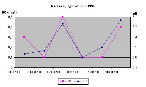
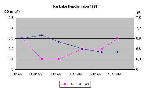
The curriculum instructs students to graph the data (manually or using a spreadsheet such as Excel). If we do this we get the following graphs:
Both graphs have to be interpreted carefully. As we have selected only
six values from the six-month period, it is unclear whether these values
depict a general trend or whether some of the values show peculiarities
and specific circumstances so that they deviate from the overall trend.
The latter hypothesis is plausible especially in the first graph where
we observe a large unusual increase in both variables in July. It is difficult
to detect the expected trend — values decreasing in summer and increasing
in autumn — in either of these graphs.
Moreover, it is difficult to judge whether the values for pH
or for dissolved oxygen should be considered as low or high because no
other values from other seasons or other layers of the lake are provided
for comparison. It could be that the pH value in winter is even less than
the value we observed in the above graphs.
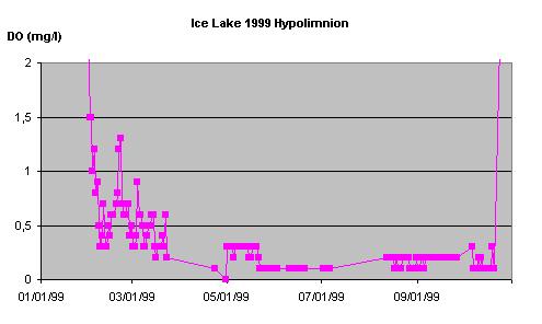
Let's look first at how dissolved oxygen varies. For the period May to October, 1998, the concentration remains below one mg/l. Near the end of October 1998 we observe a sudden increase, a trend which continues till the concentration reaches a high point of 10 mg/l. After that, the values drop back down to below one mg/l by February 1999, dropping even lower after May 1999 (0.2 - 0.3 mg/l). From June to October, 1999, they are minimal (0.1 - 0.2 mg/l). In fact, the values are so low during this period that they are about the size of the measurement error of the instrument (+/- 0.2 mg/l (http://wow.nrri.umn.edu/wow/under/qaqc.html). This can be seen more clearly in Graph 4 in which we zoom in on the 1999 data. At the end of 1999, we again see a sudden rise of the values, which remain high in the beginning of the year 2000. (The values between November and January 1999 are missing because the RUSS Unit is taken from the lake when it freezes and is reinstalled when the lake is completely frozen.)
We now look more closely at the values and compare summer 1998 to summer 1999.
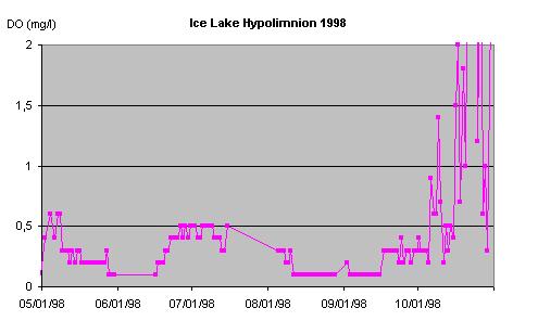
In May of 1998, the DO values decreased from 0.5 mg/l to 0.1 mg/l. From mid-August to mid-September the level was similarly low. Afterwards, there was a sudden rise. We see a similar pattern in 1999. However, there is an odd increase in DO between mid-June and mid-July when the values of DO increase to 0.5 mg/l and remain there for about two weeks. We find a possible clue in information contained in the data archive: "The data from RUSS on Ice Lake between July 1 and July 16th are suspect. We have yet to determine if the probe was malfunctioning or if the data reflect actual changes in the lake. When we determine what happened we will post our findings here." (http://wow.nrri.umn.edu/wow/data/ice/current.html) Based on this, we excluded data from this period from consideration, and even wondered whether the values observed the week earlier could also be related to this malfunction.
In summary, the DO level is very low between May and October on the bottom of the lake (nearly zero). In October of both years we see a sudden rise. The May values are a bit higher than in the following months, but still very low when compared to the winter months. Indeed, the values are so low during the summer and early autumn months that it is not possible from these data to say anything about their trend during that period. Thus, we cannot confirm in the data the expectation that the curriculum authors had hoped for, that DO trends to decrease during the summer months.
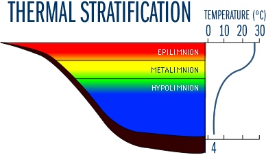
Let's extend our analysis to take into account other values of the hypolimnion as well. We refer to the the graph from lake ecology primer:
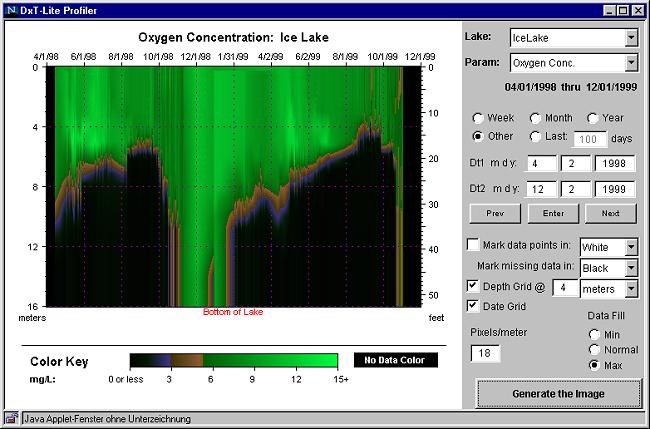
We used the DxT Profiler to generate the temperature profile of Ice Lake:
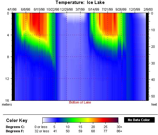
If we compare the two graphs above we see that the temperature distribution in the lake was such that we could assign water below the depth of eight meters to the hypolimnion. Based on this, we selected all DO measurements taken from a depth of at least eight meters. These are plotted in the graph below.
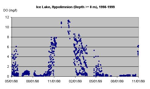
This graph gives a much clearer picture than those we have used previously.
In 1998 as well as in 1999 the expected changes can be seen: decreasing
values in May, zero level between July and October, and afterwards a steep
rise.
Another possible way to analyze the hypolimnion is provided by the
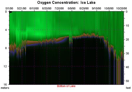
DxT profiler. We used this tool to generate the following three graphs.
The first graph shows all measurements taken since the RUSS Unit was installed
in 1998; the two other graphs show the time periods between May and November
in the years 1998 and 1999.
We can see immediately in these graphs that the DO values in the hypolimnion
are very low in the period between May and November. In the last two graphs
we also see that the blue line (corresponding to the DO level of 3 mg/l)
shifts between May and September in the direction of the surface and then
goes down again. If we assume that DO level decreases with increasing depth,
this course of the blue line exactly corresponds to the curriculum authors'
expectations.
The graphs give rise to new research questions. A peculiarity is the
two light green spots (very high DO level) directly above the brown line
in June. A new research question for the students could be to look for
an explanation for these high DO concentrations.
The above graphs lead to another critical comment concerning the "data
fill" option: this does not give unique results. In the DxT
Profiler Graphic 1 we see a bump in the blue line. This is not seen
in the next graph which is expected to be the same graph but only zoomed
in. Maybe a different algorithm generates this picture, so it is not just
a zoomed in version of the first graph. We were not able to clarify this.
pH-value
We made a similar indepth analysis for pH, but do not report that here.
However, we should mention a problem that we encountered in the process.
When we looked at the trend of pH values, we discovered some abrupt changes
(see graph below).
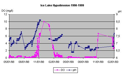
One such peculiarity can be seen at the end of May 1998 where the pH value drops from about 7 to a 6.5 (minus 0.5) and goes back to the old value after two weeks.
In the following graph, we have indicated with dotted lines the days
when the RUSS Unit was calibrated.
.
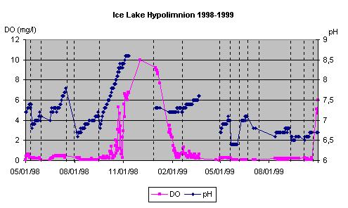
We can now see that nearly all abrupt changes, in pH in particular, coincide with the calibration of the RUSS Unit. This problem further complicates the task of interpreting the data, and should be mentioned by the curriculum authors in their materials.
Halsted Bay - Lake Minnetonka
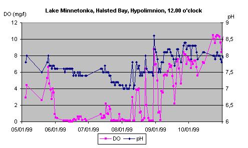
Below we report similar analyses for a different lake. Graph
7 shows values for pH and dissolved oxygen near the bottom of Halsted
Bay of Lake Minnetonka. As before, we see that the values of DO are
minimal from June to August. But we see an unexpected rise beginning in
mid-August. A hypothesis could be that some unusual event produced
the rise of DO, after which the concentration decreased back to a level
of nearly zero which would be normal. It could have been that a heavy
storm churned the water, pushing the upper layers with higher DO concentrations
downward. We can observe somewhat similar peaks in September; however,
the DO concentration does not go back to a zero level afterwards.
Based on our experience with data from other lakes, we could decompose
the unusual variation in these periods as comprising two components:
one a continuous increase due to seasonal changes, and the other these
peaks caused by special events. usua superposed by these peaks.
Obviously, it would be nice to have access to data that might confirm the
occurrence of such events.
Looking at the data using the DxT profiler, we see clearly that the DO level in the bottom layers of the lake decreases during summer and increases in autumn. However, it is unclear if this lake, which is not very deep, can be said to have layers at all so that we can reasonably speak of a hypolimnion. In August, at least, we find the same temperature in every depth (layer).
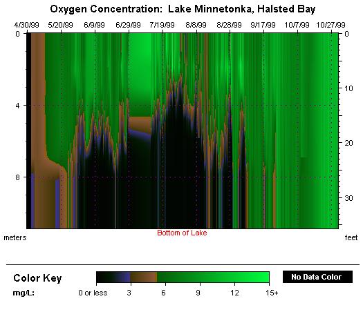
This example shows us clearly that the change of one variable is dependent on many factors. We thus should draw conclusions from particular patterns with some care.
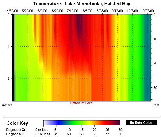
Summary:
The procedure that the curriculum suggests, of having students select six values from six months, does not give students enough data to observe the patterns that the authors hope they will observe. On the other hand, our analyses shows that the larger data provide do contain tractable patterns and the tools the project supplies (in particular the DxT profiler) are helpful in seeing these relationships. However, it should also be clear from our own analysis the time complexity involved in reasoning about these trends.
Given the limitation of looking at two variables, there are three types of questions:
A model solution for one of these questions does not yet exist, either in the teacher curriculum or in one of the students' versions. This is a severe deficiency from the perspective of data analysis, although the suggested activities are very valuable and an excellent starting point.
The "Understanding" section of the WOW website includes information about heat budgets for some WOW lakes (see Figure 1). You may want to display information such as this for the students. This could be done either during your initial discussions for this lesson, or as part of the discussion and closure for the lesson.As part of the introduction to this unit, students are asked to consider the following questions:Figure 1. Heat Budget for Ice Lake
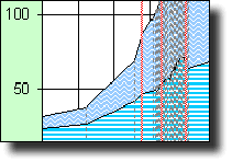
(http://wow.nrri.umn.edu/wow/teacher/heat/teaching.html)
Table 2. Water Volume and Energy Changes for Ice Lake
| Date data was collected by RUSS: ______________ | ||||||
| Water layer | Surface area of this layer (m2) | Water Volume (m3) | Temp.
change, (°C)
6am-2pm |
Calories used | Temp.
change, (°C)
6pm-2am |
Calories released |
| 0-1 m depth | ||||||
| 1-2 m depth | ||||||
| 2-3 m depth | ||||||
| 3-4 m depth | ||||||
| 4-5 m depth | ||||||
| 5-6 m depth | ||||||
Students can find a discussion of the water volume calculation as well as surface areas in Heat and Oxygen Budget , so filling in the table is a relatively easy task.
In the "investigating" lesson the students are asked to develop a similar table themselves. In both units, students are give the following 11 questions to aid them in interpreting the results:
Unfortunately, prepared graphs and data sets are not (yet) used in this
unit. To prepare graphs that allow to adequately analyze daily changes
would take some time and efforts.